mb5370

Instructors

This module was designed by me (Ira Cooke) and my colleague Prof. Matt Field. It features contributions from a number of others who we will acknowledge along the way.

Matt and I also teach a full course running in trimester 3 which provides the opportunity to learn bioinformatics in much more depth.

Preliminaries

How to read this tutorial

Command-line examples that you are meant to type into a terminal window, and the results of those examples, will be shown in a shaded code block, e.g.

ls -lrh

Sometimes the accompanying text will include a reference to a Unix command. Any such text will also be in a constant-width, boxed font. E.g.

Type the ls command.

From time to time this documentation will contain web links to pages that will help you find out more about certain Unix commands. Usually, the first mention of a command or function will be a hyperlink to Wikipedia. Important or critical points will be styled like so:

This is an important point!

So let’s dive in!

Introduction to Command-Line and RStudio

A cloud server has been provisioned for this workshop. It is a fairly powerful virtual machine but since it is needed for a few different teaching activities it will only be available to use during this workshop.

Each of you has a separate user account on this machine where you can add data, run commands and take notes. At the end of the workshop I will provide instructions on how to download this data for backup and use on other computers.

Logging in

Activity: Log in using the RStudio web interface.

Using a standards compliant web browser (Chrome, Firefox, Safari) navigate to rstudio.bioinformatics.guide. This should bring up a page asking for your username and password. You should have received these details in an email prior to the workshop.

After logging in you should see a full RStudio web interface which looks a bit like this;

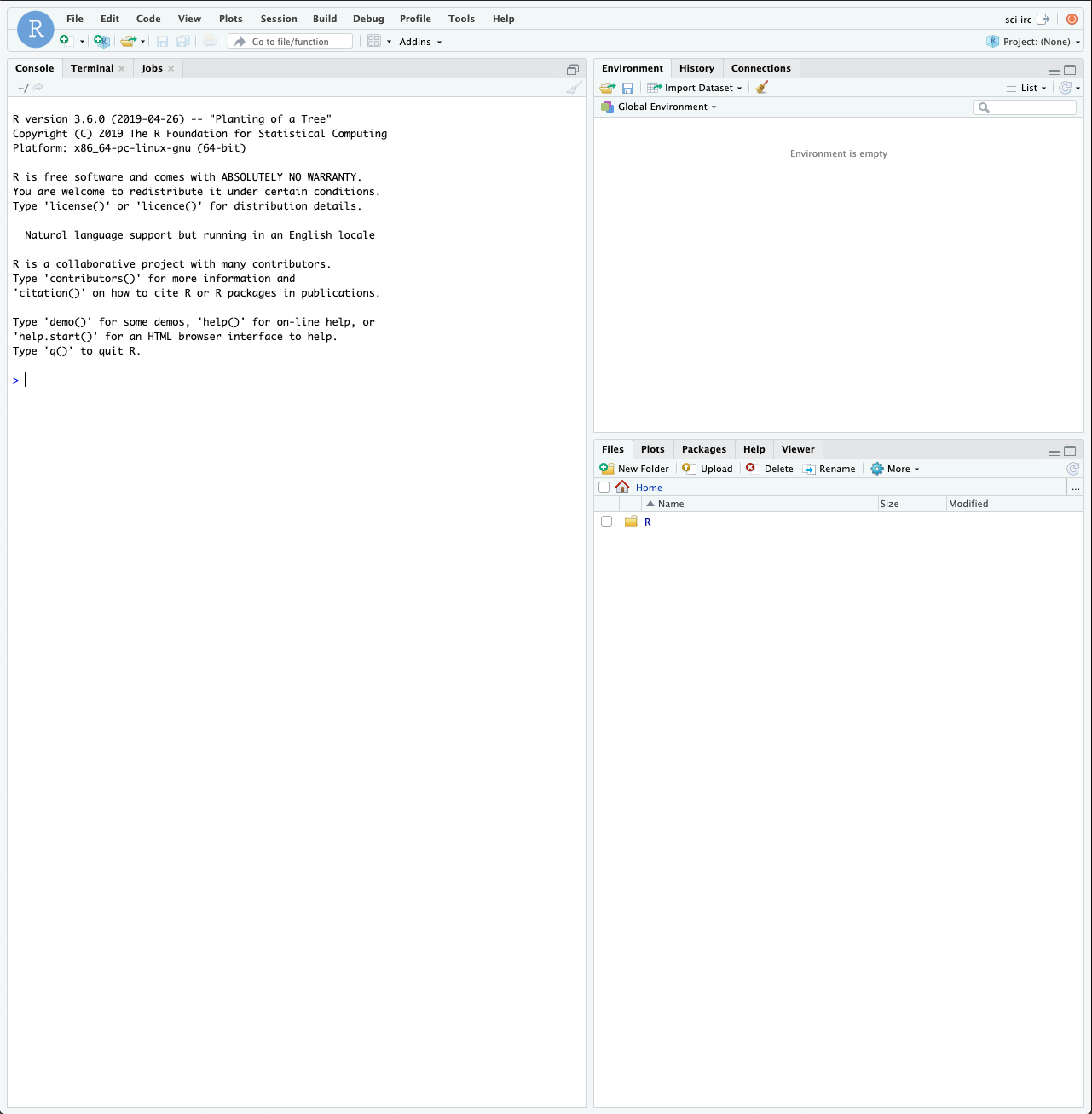
The RStudio Web Interface

Rstudio is a full featured environment for all things R. This now encompasses a very wide range of activities from interactive data analysis (R;RMarkdown) to writing R packages and even creating interactive web pages with R (Shiny).

In this workshop we will work with a web based version of RStudio. It is almost identical to the RStudio that you can download and run locally on your own laptop or desktop machine (compatible with most operating systems). For the workshop we use it simply to avoid hassles of setting things up on many people’s computers.

Another very useful feature of RStudio is its ability to interact with the underlying host operating system via the Terminal.

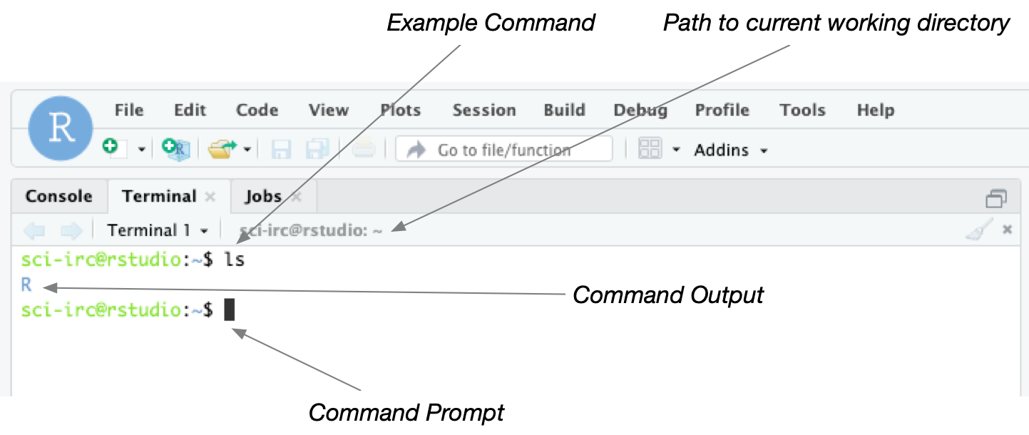
Activity: Open a Terminal Window

Click the Terminal tab in RStudio to open a command-line window. This window is where you can type unix commands. The window below shows an example. Try typing the ls command and pressing enter.

It is important to note the distinction between the Console window and the Terminal window. Both windows allow you to type commands but Console expects commands in R whereas Terminal expects unix commands.

Later in the module we will make use of the R features of Rstudio but for now we will just use it as a way to access the server and run unix commands.

Basic unix commands

While learning about the multitude of unix command line tools is beyond the scope of this tutorial we will present a few useful commands to get you started.

The Unix operating system has been around since 1969. Back then there was no such thing as a graphical user interface. You typed everything. It may seem archaic to use a keyboard to issue commands today, but it’s much easier to automate keyboard tasks than mouse tasks. There are several variants of Unix (including Linux), though the differences do not matter much for most basic functions.

Unix is particularly suited to working with biological sequence files, even very large ones, and has several powerful (and flexible) commands that can process your data for you. The real strength of learning Unix is that most of these commands can be combined in an almost unlimited fashion. So if you can learn just five Unix commands, you will be able to do a lot more than just five things.

Unix file system

In unix files are stored in a tree structure.

Understanding where you are in this tree is critical when using the command line and usually the single biggest source of confusion for these workshops!

So where am I?

Let’s try our first command pwd (print working directory) which addressed this issue:

Activity: First unix command. Type pwd in the terminal.

This shows your path within this tree. You’ll never be lost again!

What just happened? When we type pwd into the shell several things occur:

1) finds a program called pwd

2) runs that program

3) displays that program’s output, then

4) displays a new prompt to tell us that it’s ready for more commands.

Unix command format

pwd is a simple command that takes no arguments however in general unix commands have up to three components:

1) The command name

2) The flags or modifiers -> changes default behavior

3) The arguments -> input files, etc

Let’s illustrate using the ls command, a command that tells us what is present in our current directory.

Activity: Type ls in the terminal.

This shows us any files and directories present in our location.

Now try adding the -l flag (long format)

ls -l

Now we see more information for each file/directory.

Now try adding the -r flag (reverse sort)

ls -lr

Notice how we combined the flags?

That’s the concept behind flags but what about the argument?

By default ls displays information in the current directory but we can change this by passing in a different directory. Try it!

ls -l /usr

Instead of your current directory, the command queries the /usr directory.

That explains the concept of commands, flags and arguments

Other useful unix commands

Create directory

If we want to make a new directory (e.g. to store some work related data), we can use the mkdir command (Tip: don’t use spaces when naming):

Activity: Create directory

Lets try it!

cd
mkdir command_line
ls

We see the new directory has been created.

Moving around

We are in the home directory on the computer but we want to to work in the new command_line directory. To change directories in Unix, we use the cd command as you might have observed above:

Activity: Change directory

cd command_line

Remember that you can always find out where you are using pwd:

pwd

We are in the new directory and see the full path

View file contents

Now copy the following to create a mock fasta (don’t worry about details for now).

cd ~/command_line
echo $'>fasta_header\nMMGTSRCVILLFALLLWAANAAPPEIHTTRPNVPEEIKRPNSTEIETPAVKQLETPSIFL\nLTTLEVAEADVDSTLETMKDRNKKNSAKLSKIGNNMKSLLSVFSVFGGFLSLLSVVTTTS' > test.fasta

Now let’s have a look at the file using the command cat

cat test.fasta

What about if the file is huge and we only want to view the first few lines? Use the head command.

head -2 test.fasta

By default head will display the first 10 lines but the -2 only displays the first 2 lines

Search for specific content in files

Lastly we’ll show you powerful command grep (globally search a regular expression and print)

grep finds lines matching specific strings in files.

Activity: Learn about grep

For example if we want to find the fasta header (make sure to include the quotes in this command!).

grep '^>' test.fasta

If we want to find a specific amino acid sequence:

grep KDRNKKNSAK test.fasta

Grep has many useful flags. Use the man command to view some of the flags.

man grep

grep has roughly 50 flags!

Some of my favorites include:

1) -i -> case insensitive match

2) -n -> report line number of matches

3) -c -> report all files that contain the pattern

4) -w -> match whole words only

Let’s try adding the line number with the ‘-n’ flag

grep -n KDRNKKNSAK test.fasta

Now we see the line number included.

That should give you a taste of a few basic unix commands, hopefully you can pick the rest up as you go.

And finally….

Remember to check where you are before running commands!!!!

Beyond default commands

Beyond the built in unix commands you launch installed applications.

For example to run firefox you can simple type firefox on the command line (don’t do this now).

You can even install new programs and run them from the command line.

For example, later we will use a program called bioawk. It has been installed for you.

Projects and Files

A great way to organise your work when using RStudio is to create a Project. This is essentially just a folder with a special .proj file in it. When you open the .proj file RStudio will set things up so that you can easil work with files inside the project folder.

Activity: Create an RStudio project

Create a new RStudio project. This project will contain all the scripts you create for this workshop. Since this is the first workshop and it is largely about learning unix commands a sensible name would be workshop1_unix. Throughout the genomics module you will often be instructed to give files and folders certain names. Although you are free to choose your own names (in theory), in practice you are less likely to run into trouble if you stick to the names we provide. Commands and examples we give will assume you named your files as instructed.

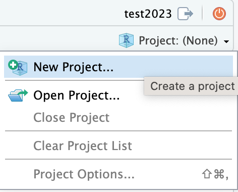
To create the project use the project menu at the top right of the RStudio interface

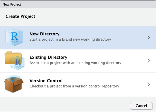
Then select new directory as the project type, and then New Project again in the menu that appears

Activity: Explore the location of project files and folders

After creating the new project RStudio will automatically open it. In doing so it will change your current working directory to the workshop1_unix directory.

Open the Terminal window in RStudio and use the unix commands ls, pwd, and cd to explore files and folders on your system.

Activity: Create another new project and try switching between them

The project menu at the top right of RStudio allow you to easily switch between projects. Creating multiple projects will give you a feeling for what exactly a project is (ie just a folder with a .proj file) and what it means to switch between or open a project.

Make sure you switch back to the workshop1_unix project after you are finished experimenting with new projects.

RMarkdown

When starting out in bioinformatics many people take notes in document editing programs familiar to them such as Microsoft Word. While this can sometimes work it is much better to take notes using a plain text format. Programs like Word are terrible for writing computer code because they will do unexpected things like capitalize words or convert characters (eg convert a double dash -- into a longer single hyphen).

Markdown is a simple plain text format that is great for taking notes and writing larger documents that include computer code. RMarkdown is a variant of Markdown that is understood by RStudio and allows you to include code chunks that can be run to create images or perform analyses.

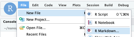
Activity: Create an RMarkdown file for taking notes.

Create a new file using the File menu in RStudio. Note that the first time you do this RStudio will prompt you to install a bunch of packages. Just click OK to install them.

Call it Command Line Basics and select output format as html. After RStudio has created your document you should save it. Name the file 01_basics.Rmd.

Naming conventions are a very important organisational tool. I like to name all my files using a numeric prefix within projects. This provides a sequential order to things that I find is often helpful when tracking down what I have done.

Activity: Note down some commands

So far today we have used the, ls, cd, pwd commands. Make some notes about these in your newly create RMarkdown document.

First delete the placeholder text that comes with the template document. This means everything below the heading ## RMarkdown but not the code chunk and title field above it.

For full details on how to author RMarkdown documents refer to the cheat sheet.

When you have made some edits click the Knit button to see what your document looks like as an html page

Moving files to/from the remote server

At some point you are likely to want to either copy your files from the rstudio server down to your laptop or vice versa. This can be done using rstudio as follows;

You can export selected files which will zip them up and download them to your computer

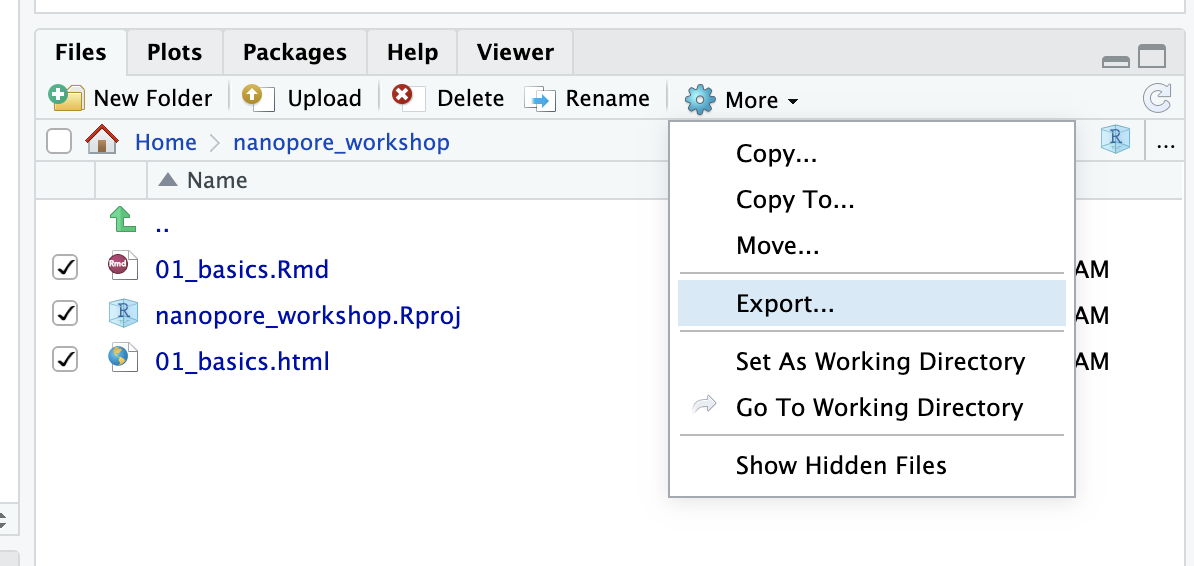
In the other direction you can use the Upload button to upload files from your laptop

Sequence File Formats

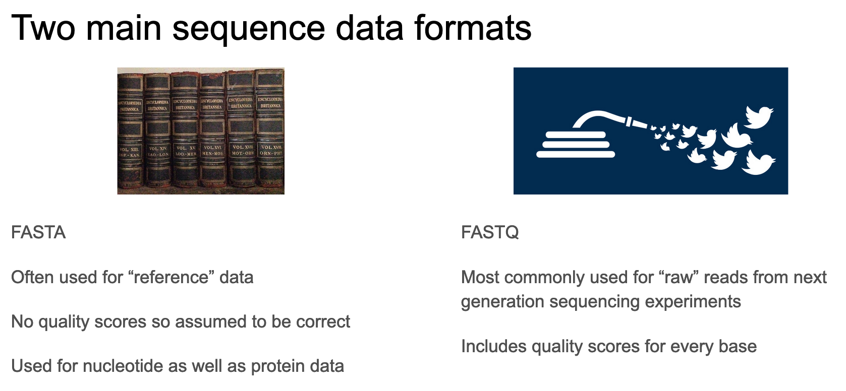
We created a fasta file in the previous section but let’s look closer at fasta and fastq formats.

These are the two common formats for storing sequence information. How do they differ?

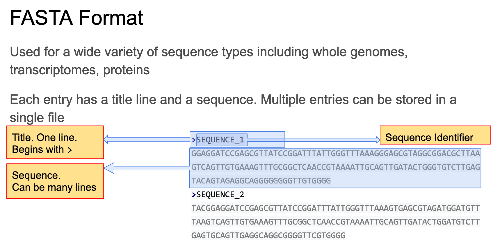
Now let’s consider fasta

The fasta format consists of 1 or more entries each of which consists of a header and a sequence

The fastq format is designed for storing sequencing data along with quality scores.

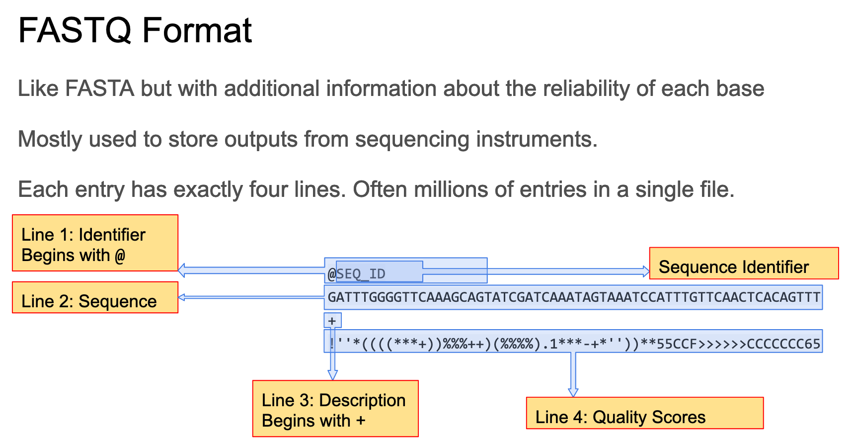
It is a standard format used for many types of sequencing including Illumina short reads and longer reads produced by Nanopore or PacBio sequencing. See this wikipedia page for a more detailed description of the fastq format.

Each read occupies 4 lines in a fastq file. The lines are as follows;

1. Starts with @ and contains a unique identifier for the sequence
2. Is the sequence itself
3. Starts with + and almost always nothing else
4. Contains quality scores. These are encoded using ASCII characters with one character per base.

The full list of qualty score letters from 0-94 is

!\"#$%&\'()*+,-./0123456789:;<=>?@ABCDEFGHIJKLMNOPQRSTUVWXYZ[\]^_\`abcdefghijklmnopqrstuvwxyz{|}~

End of Preliminaries.

That takes you through the basics of Rstudio, unix and sequence formats.

If you want more practice with command-line basics I recommend you run through the 30 minute tutorial at terminal tutor.

Now move on to workshop 2, genome assembly