mb5370
Welcome!
I hope you enjoy this workshop on genome assembly. The first version of this workshop was developed by Assoc. Prof. Ira Cooke but it has since been refined by Dr. Andrew Calcino, Dr. Sally Lau and Prof. Matt Field.
For this exercise will use data from a previous MinION run on a culture dominated by a bacterium in the genus Vibrio. The dominant organism has two large chromosomes with sizes around 3.4Mb and 1.8Mb respectively. We also expect some smaller plasmids. At very high coverage it was also revealed that this data contained another bacterium (a Gammaproteobacterium) which was around 100 times less abundant than the Vibrio.
Create a new project
Start by creating a new project in RStudio for this workshop. Name your project workshop2_assembly.
All of your work for today will go in this project folder. All of the commands you will run today assume that you are working from within this project folder. After you have created your project open a Terminal window and check that you are in the right place
pwd
When you run this command it should print something like /home/jcXXX/workshop2_assembly, where jcXXX is your JCU login ID.
Next, create a new RMarkdown notebook to take notes on the commands you will run today. I recommend saving it using the filename 01_assembly.Rmd
Redbean Assembly
Assemble a genome with redbean
We will start by using one of the fastest long read genome assemblers, which is now called redbean, likely because the original name WTDBG2 was just plain terrible. This software is available from github at https://github.com/ruanjue/wtdbg2. Lucky for you, redbean has been preinstalled here but if you would like to try install it yourself on your own machine at another time, we recommend a manual installation from the github repo because the conda version is out of date.
First prepare a directory for running the software using the mkdir command
mkdir redbean
Then use the cd command to change into this directory.
cd redbean
Collect a small subset of data for the initial assembly. We will use just the first 3 files which equates to 12000 reads and around 6x coverage of the target genome. This will almost certainly not be enough to generate a good assembly. As a learning exercise it will be useful to compare the results with this small dataset to results we will obtain later using more reads.
cat /pvol/data/amtp4/*_[012].fastq > amtp4.fastq
Run the assembly
wtdbg2 -x ont -g 5m -t 4 -i amtp4.fastq -fo amtp4
wtpoa-cns -t 4 -i amtp4.ctg.lay.gz -fo amtp4.ctg.fa
Take a rough note of how long this assembly takes.
Activity: Inspect assembly statistics
assembly-stats amtp4.ctg.fa
How good does the assembly look in terms of contiguity and completeness? These concepts were covered in lecture 6.4
Run redbean with higher coverage
Now let’s redo the assembly using a better coverage depth. We will use data equivalent to around 20x coverage.
cat /pvol/data/amtp4/*.fastq > amtp4_20x.fastq
wtdbg2 -x ont -g 5m -t 4 -i amtp4_20x.fastq -fo amtp4_20x
wtpoa-cns -t 4 -i amtp4_20x.ctg.lay.gz -fo amtp4_20x.ctg.fa
Using this larger dataset redbean takes around 13 minutes
Activity: Inspect assembly stats for higher coverage
Reassess the assembly using assembly-stats.
Flye Assembly
Now we will try an alternative assembler called Flye. This assembler has been around a bit longer than redbean and is a more mature software project. As far as long read assemblers go it is fairly quick but not as fast as redbean. Again, lucky you, it has already been installed on your system but if you want to try it out on your own machine later, you can go with the conda version for flye.
Setup a Flye working directory
Before we run the assembly using Flye we need to setup a directory where we will store the outputs and run commands.
First confirm that you are in your redbean directory.
pwd
This should show /home/jcXXX/workshop2_assembly/redbean. If not then you will need to move (with cd) to your redbean directory before running the commands below.
Next move “up” a directory using the command
cd ..
Here .. means the directory “above” the one we are currently in. Now run pwd again. This time it should show /home/jcXXX/workshop2_assembly/.
Now you are ready to make the flye directory and cd into it.
mkdir flye
cd flye
Finally. Double-check that you are in the right place. pwd should give /home/jcXXX/workshop2_assembly/flye
Run Flye on both datasets
Make symbolic links to the same raw data we used for redbean
ln -s ../redbean/amtp4.fastq .
ln -s ../redbean/amtp4_20x.fastq .
Start by running Flye on the smaller dataset. Even this will take quite a while (about 15 minutes). We would like to keep working while flye runs in the background and we would also like to make sure that even with lots of us running Flye at the same time we don’t overload the server. To deal with these issues we will run flye using a queuing system called slurm. Systems like slurm are normally used in large clusters or supercomputers and can prioritise large numbers of jobs across many compute nodes. The JCU High Performance Computer system (JCU HPC) uses a similar system called PBS. Here I have installed slurm on our single node to allow the whole class to run longer jobs without crashing the server.
To run a command as a slurm job requires a little extra effort. Instead of simply typing the command in the Terminal and hitting enter we need to wrap our command into a short “job script”. This script is a separate file where we will include instructions about how much memory and CPUs we need as well as the command to run.
Create a new empty shell script file for your slurm script
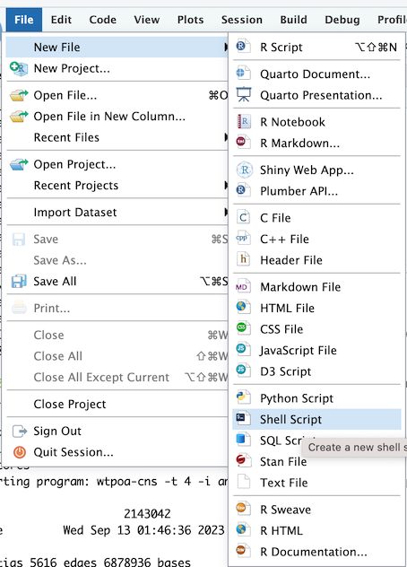
Save your file inside the flye directory and call it run_flye_small.sh

Now cut and paste the following text into your file and save it
#!/bin/bash
#SBATCH --time=60
#SBATCH --ntasks=4 --mem=4gb

echo "Starting flye in $(pwd) at $(date)"

flye --nano-raw amtp4.fastq --out-dir amtp4 --genome-size 5m --threads 4

echo "Finished flye in $(pwd) at $(date)"
Once you have saved your slurm script you can submit it to the queue using the sbatch command
sbatch run_flye_small.sh
When you run this you should see a result like Submitted batch job XXX where XXX is a number.
It is really important that you only run this sbatch command once or you might end up with multiple conflicting runs of flye trying to overwrite each other.
You can check the status of your job (and everybody elses) by running squeue.
squeue
Once your job starts you should see a new file in your flye directory called slurm-XXX.out (where XXX is your job number). Have a look at this file.
tail slurm-XXX.out
It shows output from the flye command as it is running. If you want to follow (-f) the output as it is created use
tail -f slurm-XXX.out
Activity: Monitor running jobs
You can use the squeue command to see the jobs that are running. This should show your instance of flye. You can look for it with your username.
Also try top which shows all the most CPU intensive tasks being run by the entire system. Here you should be able to see everybody’s flye processes.
Activity: Assess assemblies made using Flye
Once flye has finished, the final assembly will be available inside the output directory and will be called assembly.fasta. Use the assembly-stats program to assess the contiguity and completeness of this assembly.
Now run flye on the larger dataset. This will take a very long time. We will come back to it later.
To do this make another new shell script file and save it into your flye directory. This time call it run_flye_large.sh. Cut and paste the following code into your shell script
#!/bin/bash
#SBATCH --time=360
#SBATCH --ntasks=4 --mem=4gb

echo "Starting flye in $(pwd) at $(date)"

flye --nano-raw amtp4_20x.fastq --out-dir amtp4_20x --genome-size 5m --threads 4

echo "Finished flye in $(pwd) at $(date)"
After the large assembly has finished assess it with assembly-stats and look at its GFA file with Bandage (see below).
Inspect assembly graphs with Bandage
One of the nice features of Flye is that it produces output in the GFA format. We can use a nice graphical tool called Bandage to inspect GFA files.
Activity: Inspect low coverage flye assembly with Bandage
First download and install bandage. It is available for all major operating systems.
Look inside the output directory for the first flye run. Find the file called assembly-graph.gfa. Use RStudio to download this file to your laptop.
Now open bandage and use the File->Load Graph menu to load the file assembly-graph.gfa. Then click Draw Graph.
In this visualisation contiguous segments are shown as solid coloured lines. Some of these are separated into independent graphs whereas others (eg the mess in the top left) are connected to each other via black lines. There are few things to keep in mind here;
- Biologically distinct entities such as chromosomes or plasmids will form separate graphs
- Separated graphs can also occur if coverage is very low and no reads exist to join parts of the assembly together
- Highly joined regions (eg top left) tend to occur because repeats create ambiguities. There are too many connections and the assembler has trouble choosing the correct path between them.
Try zooming in on the highly connected region. Click and move contigs around to get a clearer look. Clicking on a contig shows the depth of read coverage assigned to it. Based on read coverage and the shape of the graph can you spot a segment that might correspond to a repeat?
Activity: Inspect high coverage flye assembly with Bandage
Repeat the exercise above using the high coverage (20x) assembly generated with Flye. Can you spot the same repeat region? How has increased coverage changed the appearance of the assembly.
Which contigs look like fully assembled chromosomes? Which ones look like plasmids?
Check Assembly Quality with QUAST
Up to this point we have performed four separate assemblies with 2 different assemblers and 2 different levels of coverage. Although we could clearly see a huge improvement in contiguity with the addition of more reads we could not easily check for the accuracy of assemblies.
For this particular example we have a reference assembly which we previously created using very deep coverage and best-practice genome polishing tools. By comparing our assemblies to the reference we can assess them in terms of all the important metrics, contiguity, completeness and correctness.
Setup a Quast working directory
Hopefully this will be starting to seem familiar. First check that you are in the flye directory. Run pwd in Terminal. It should show something like /home/jcXXX/workshop2_assembly/flye.
Next cd up to the directory above with
cd ..
Then make a directory for quast and cd into it
mkdir quast
cd quast
Prepare assembly data
Now make two directories within the quast directory. These will be used to store our assemblies from flye and redbean
mkdir flye_asm redbean_asm
Our reference assembly only contains contigs for the two major Vibrio chromosomes. For our two deeper coverage assemblies this will correspond to the two largest contigs. We extract these (and ignore all others) in order to make the assembly comparison easier to interpret.
Use this command to look at the contig sizes in the flye assembly
cat ../flye/amtp4_20x/assembly.fasta | bioawk -c fastx '{print $name, length($seq)}' | sort -n -k2
For me this was contig_11 and contig_56 but these numbers may differ from assembly to assembly. Use samtools to extract these
samtools faidx ../flye/amtp4_20x/assembly.fasta contig_XX contig_YY > flye_asm/vibrio.fasta
Now that you will need to modify this command by replacing XX and YY with the contig numbers of the two longest contigs in your assembly.
Now repeat the process for the redbean assembly
cat ../redbean/amtp4_20x.ctg.fa | bioawk -c fastx '{print $name, length($seq)}' | sort -n -k2
samtools faidx ../redbean/amtp4_20x.ctg.fa ctg1 ctg2 > redbean_asm/vibrio.fasta
Now create a symbolic link to the original reads
ln ../flye/amtp4_20x.fastq .
We also need the reference assembly so make a symbolic link to that as well
ln -s /pvol/data/amtp4/reference/vibrio .
Run QUAST
Run quast as follows
quast -o quast_vibrio redbean_asm/vibrio.fasta flye_asm/vibrio.fasta -L -t 4 --circos --glimmer -r vibrio/vibrio.fna --features vibrio/vibrio.gff --nanopore amtp4_20x.fastq
Activity: Inspect quast outputs
Quast outputs should be saved to a folder called quast_vibrio. Download this folder to your laptop and unzip it. Some things to look at include
- The main report
report.html - A circos plot in
circos/circos.png
Both assemblers seem to have done a very good job of assembling the genome but both have produced regions where there are a large number of small differences (snps and indels) between the assembly and the reference. The redbean assembly also seems to have a couple of gaps which most likely correspond with the highly repetitive region we observed in the Bandage visualisation.
Optional: Check final assembly for adapters
Notice that we didn’t actually do any adapter trimming prior to running flye or redbean. In a real project we would probably run porechop on all the reads to trim adapters. This would most likely improve the assembly and reduce the possibility of incorporating adapter sequences into our final product.
As an exercise use porechop to check for adapters in the various assembly files you created.
Good to do when you have time: Polishing the assembly
Although long reads provide very high contiguity they generally have low accuracy. To a large extent this low accuracy can be overcome obtaining a high read depth and taking the consensus of many reads at each position. Some genome assemblers incorporate such error correction (eg Canu) but even in such cases it is always a good idea to use a dedicated assembly polishing tool to correct small errors in the assembly.
A good polishing tool for Oxford Nanopore data is medaka. Ideally we would probably want some more accurate Illumina data for final polishing, or PacBio data which has less biased errors than Nanopore. For each of these tasks there are a growing number of programs that can be used.
Mystery Repeat Region - Only complete if we have time
We have just shown with ‘bandage’ that the ‘flye’ assembly contains a repeat region that could not be completely resolved. Let’s have a look and see what might be going on here.
For this exercise we will run commands and store results in a directory called repeat. Assuming that you are in your quast directory, you would run the following commands to set this up and cd into it.
mkdir ../repeat
cd ../repeat
Extract repeat region sequence
Use bandage to extract the repeat region as follows;
- Click on the repeat to select it
- Use the
Outputmenu to copy the repeat sequence to your clipboard - In rstudio, open a new blank text file and paste in the sequence
- Edit the text file to add a fasta header line (see below) with the text
>repeat_1 - Save the file into
repeat/repeat.fasta
Use prokka to annotate it
Now run prokka on this sequence to see if it contains any transcribed sequences
prokka --outdir prokka --prefix repeat repeat.fasta
Now look at the tsv file that is produced. What type of genomic features dominate this sequence?
cat prokka/repeat.tsv
Genomic arrangement of repeats
Now we know the genes that are present in our repeat but we don’t know how the repeats are arranged in the genome. Specifically we are interested in whether they are arranged in tandem or dispersed throughout the genome.
To investigate this we can map the repeat sequence back to the genome itself. The tool of choice for mapping long reads and/or long DNA sequences is minimap2
Run the alignment
Link in the data
ln -s ../quast/vibrio/vibrio.fna .
Run minimap2. There are many ways to run minimap2. A great resource to help figure out which options to use is the minimap2 cookbook. In this case we are using minimap2 in much the same way as we would use to map reads.
minimap2 -x map-ont vibrio.fna repeat.fasta > repeat_vs_genome.paf
Examine the alignment
Try looking at the first few lines of the paf file that was produced.
head repeat_vs_genome.paf
It looks complicated but is just another tab separated format. The format is described on this webpage. The first 12 columns are standard but more columns may be present (documented elsewhere).
For our purposes the important columns are those specifying the start and end point on the target. We can extract these columns into a bed formatted file as follows;
cat repeat_vs_genome.paf | grep '^repe' | awk -F '\t' '{print $6,$8,$9}' > repeat_locations.bed
Question?: Is this a tandem repeat or interspersed?