mb5370

In this workshop we will assemble a mock metagenome consisting of five bacterial species. Compared with a real metagenome this community is very simple, however, it has been designed to capture some of the key challenges inherent in metagenomic assembly, namely;

• Variable coverage: Some species are very abundant whereas others are quite rare. Assembling the rarer taxa is more difficult.
• Similar sequences: This community contains two Vibrio species. These are similar enough that they are difficult to separate in an assembly

The table below shows the relative abundance (Proportion of Reads) of each species in our mock community. Since this is a mock community we already have reference genomes for each member. Information on each genome can be found by typing its accession (eg. ASM31704v1) into the search field on the NCBI database of microbial genomes.

For the purposes of metagenomic assembly we note the number of chromosomes, total genome size and its GC content. We will use these pieces of information later to assess our preliminary assembly results.

Proportion of Reads	Species	Accession	Number of Chromosomes	Size	GC Content
44.5	Geitlerinema sp. PCC 7407	ASM31704v1	1	4.7Mb	58
30	Vibrio alfacsensis	ASM1967048v1	2	5.3Mb	44
7.5	Vibrio algicola	ASM960176v2	3	3.5Mb	42
15	Desulfovibrio sulfodismutans	ASM1337645v1	2	4.4Mb	63.5
3	Winogradskyella schleiferi	ASM1339465v1	1	4.6Mb	34.5

Workshop outline

In this workshop we will proceed through a full metagenomic assembly. Some of this will be familiar as it is similar to assembling a single bacterial genome, however, there are two additional steps, Binning and Bin assessment that are unique to metagenome assembly.

1. Examine Reads
2. Assembly
3. Basic assembly QC
4. Binning
5. Bin assessment

At each step you will be guided through the commands you need to run for the analysis. Each step also has exercises and questions designed to test and extend your knowledge.

Important: After you have finished these steps for the mock metagenome community you will need to repeat the process for real long-read sequencing data of black band disease.

Step 1: Examine Reads

Input data for this exercise consists of simulated reads from an Oxford Nanopore MinION sequencer. Later in the workshop we will work with real data, but for now we will use this simulated data. In case you are curious, the data were simulated using a program called Badread with parameters designed to imitate the characteristics of Oxford Nanopore’s latest chemistry.

Start by creating a new RStudio project for this workshop. Make sure you name your project workshop3_metasm and make it a subdirectory of your home directory.

After you have created this project make a new subdirectory called raw_reads. Then make a symbolic link to the raw reads file in this directory.

mkdir raw_data
cd raw_data
ln -s /pvol/data/metagenome_assembly/reads_R10_0.5.fastq.gz raw_reads.fastq.gz

After you have done this you should change directory back “up” out of raw_data like this

cd ..

Now you can check that your files are correct by using the ls command to list all files and directories in your project. Use the -l option to show extended details on each file which will allow you to see the source and target paths for the symbolic link. The resulting output should look similar to that shown in the screenshot below. Note that you will see your jc number instead of sci-irc which is mine. You will also see different dates on files which is also fine.

ls -lR .

Documenting your work

Create a new RMarkdown file and save it with the name 01_metagenome_assembly.Rmd. Use this document to take notes on the commands you run. You can document bash code, R code and also include plain text in this file.

Read Length Distribution

During the assembly process we will take shorter sequences (reads) and attempt to join them together into longer sequences. One of the most important determinants of success in this process is the size of the raw reads themselves. Our starting point for this assembly is to examine the read length distribution in our input data. If you remember back to workshop 2 we did this already for the bacterial isolate data. We will repeat the process here for our simulated metagenomic reads.

zcat raw_data/raw_reads.fastq.gz | head -n 40000 | bioawk -c fastx '{print $name,length($seq)}' > read_lengths.txt

This command consists of four parts chained together. These parts are explained below (don’t run the code below. It is for explanatory purposes only)

# Unzips the raw data and sends the data to standard output
zcat raw_data/raw_reads.fastq.gz \
# This is a pipe. It sends output from the previous command as input to the next command
  | \
# Here we select only the top 40k lines in the file. This equates to 10k reads. It should be plenty to get some stats
  head -n 40000 | \
# This is a small bioawk program. It prints the name of each sequence followed by its length
  bioawk -c fastx '{print $name,length($seq)}' \
# Send outputs to a file called read_lengths.txt
  > read_lengths.txt

Now let’s create a plot to visualise these read lengths. Note that the code below is actually R code not bash. Enter it into an R code chunk in your RMarkdown document.

library(tidyverse)

rl_data <- read_tsv("read_lengths.txt",col_names = c("id","length"), show_col_types = FALSE)

ggplot(rl_data, aes(x=length/1000)) + 
  geom_histogram(binwidth = 2) +
  xlab("Read Length Kb") + ylab("Number of Reads")

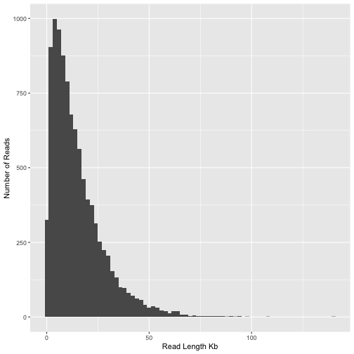
Figure 1: Histogram of read lengths in the mock nanopore sequencing dataset

Calculating read N50

From this plot it is clear that the majority of reads are between 1 and 50kb in length. A good way to summarise this is the N50 statistic. Although N50 is most often used to summarise genome assemblies it’s also very useful for summarising read length distributions. The reason this statistic is useful is because it is unaffected by having a large number of tiny reads and instead places greatest emphasis on the longer reads in the data. Let’s calculate the read N50 for our sample of reads. The method we will use to calculate N50 is described by the following pseudo-code

• Step 1: Rank all reads from longest to shortest
• Step 2: Create a new column with the cumulative sum of read lengths (starting from longest read).
• Step 3: Find the read at which the cumulative sum surpasses 50% of the total read volume (ie total sum of all read lengths)

total_len <- sum(rl_data$length)

rl_data %>% 
  arrange(desc(length)) %>% 
  mutate(cumsum = cumsum(length)) %>% 
  filter(cumsum>total_len/2) %>% 
  head(n=1)

## # A tibble: 1 × 3
##   id                                        length   cumsum
##   <chr>                                      <dbl>    <dbl>
## 1 c96c1300-8177-e260-d9bd-2fdf75d0146b_2040  22322 74486252

Activity (optional) : Pick apart and understand the code above

Break up the code in the snippet above. Start by removing all pipes and slowly add them back, looking at the data each time. Make sure you understand what the code is doing.

We see here that the the N50 of the individual reads is about 22Kb. Keep this in mind as we perform assembly. We expect that the N50 of our assembly should be considerably greater than this.

Step 2: Assembly

Assuming that we are satisfied with the overall quality of our reads the first step is to assemble them. We will use flye for this task because it is probably the best assembler for long-read metagenome data.

First make a flye directory in your project folder.

mkdir flye

Change directory (cd) to this new flye directory. We will run all flye commands from within this directory.

cd flye

Run flye on the simulated data. Running this command could take a while (~20 minutes) so we will wrap it up into a slurm job script. Hopefully you will be familiar with this now from workshop 2.

1. Create a new shell script called run_flye.sh and save it in the flye directory

2. Add the following code to your script (cut-paste)

   #!/bin/bash
   #SBATCH --time=360
   #SBATCH --ntasks=8 --mem=4gb
      
   echo "Starting flye in $(pwd) at $(date)"
      
   flye --nano-hq ../raw_data/raw_reads.fastq.gz --threads 8 --out-dir mock --meta
      
   echo "Finished flye in $(pwd) at $(date)"
   

3. Submit your job using the sbatch command

   sbatch run_flye.sh
   

4. Monitor job output

   tail -f slurm-XXX.out
   

Activity: Flye will report the read N50. How does this compare with the value we computed earlier?

While flye is running you can keep working. A good thing to do while you wait is to complete the section on calculating chromosome lengths and GC content within our reference data. After flye is finished running we will compare these results with those of our newly assembled metagenome.

Once finished, outputs from flye will be available in the directory mock. The key output files are;

File	Description
assembly.fasta	The actual assembled contigs
assembly_graph.gfa	Representation of the assembly graph in gfa format.
assembly_graph.gv	Assembly graph in graphviz format
assembly_info.txt	Table of information on each contig

Activity: Visualise the assembly using bandage

Question 3.1

What is the size and coverage of the largest contig in the assembly?

Question 3.2

Your assembly should contain at least one (probably several) large circular contigs. Based on size and coverage can you guess which contig corresponds to the genome of the most abundant species in our mock community?

Chromosome lengths and GC content in the reference data

When flye is finished running we will want to compare the assembled contigs with reference genomes from the 5 species that comprise our mock community. We will do this here in a very crude way just by tabulating chromosome lengths and their corresponding GC content.

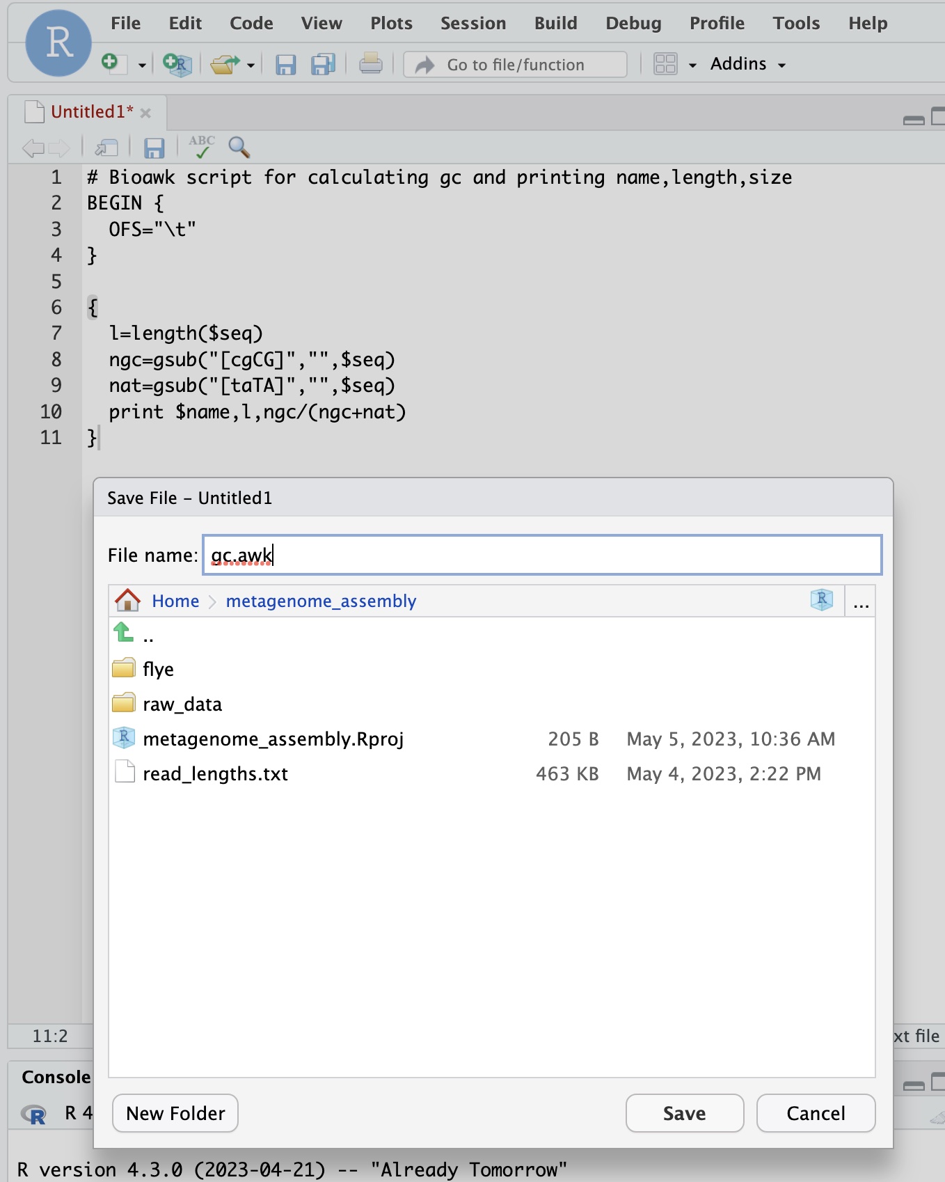
The code below shows a bioawk program for calculating GC content and size. Create a new plain text file in rstudio and paste this code into it.

# Bioawk script for calculating gc and printing name,length,size
BEGIN {
	OFS="\t"
}

{
	l=length($seq)
	ngc=gsub("[cgCG]","",$seq)
	nat=gsub("[taTA]","",$seq)
	print $name,l,ngc/(ngc+nat)
}

Save your new file with the name gc.awk in the top level of your project directory

All the reference genomes for our mock community can be found at the path /pvol/data/mg/refs/. Take a look with ls

ls /pvol/data/mg/refs/*.fna

Now test your awk program by using it to print the GC content and contig lengths for all chromosomes in these files. Here we use cat to concatenate all the files together and then use a pipe to send their contents to our bioawk program

cat /pvol/data/mg/refs/*.fna | bioawk -c fastx -f gc.awk

Question 3.3

Locate two circular chromosomes for Vibrio alfacsensis in bandage. Use the outputs from gc.awk to help with this.

Step 3: Basic Assembly QC

Make sure your flye assembly is finished and that you have completed step 2 before proceeding.

Previously we used gc.awk to print the length and GC content for reference sequences. Now we will do the same thing for our assembled contigs.

First make a new directory and change into it.

mkdir assembly_check
cd assembly_check

Use your gc.awk script to print GC and lengths for the assembly

cat ../flye/mock/assembly.fasta | bioawk -c fastx -f ../gc.awk 

Run the command again but this time send outputs to a file called assembly.gc.tsv.

cat ../flye/mock/assembly.fasta | bioawk -c fastx -f ../gc.awk > assembly.gc.tsv

Now let’s create some plots in R to explore the GC content and coverage depth of contigs. Remember that in a real metagenomic assembly we would not know the reference sequences and we would like to be able to group contigs from the same species together. Two of the most useful statistics for this purpose are the GC content and the coverage depth because these should generally be similar for contigs derived from the same chromosome.

We have GC content in assembly.gc.tsv and coverage depth in the assembly_info.txt file produced by flye. Let’s read those and join them together using R.

gc <- read_tsv("assembly_check/assembly.gc.tsv",col_names = c("#seq_name","length","GC"))
info <- read_tsv("flye/mock/assembly_info.txt") 

Since both datasets have a #seq_name column we can join them easily as follows

gc_info <- info %>% 
  left_join(gc)

A histogram by GC content shows several peaks, probably corresponding to major groupings of taxonomically distinct lineages within the data.

gc_info %>% 
  ggplot(aes(x=GC)) + geom_histogram() + ylab("Number of contigs")

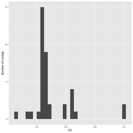
Figure 2: Histogram of GC content values values for assembled contigs in a flye assembly of the mock community dataset.

A plot of GC vs coverage helps to identify clusters that have similar values for both these parameters. In making this plot we first filter the data to remove contigs with unrealistically high GC content and very high coverage depth (probably repeats)

gc_info %>% 
  filter(GC<0.8) %>% 
  filter(cov.<25) %>% 
  ggplot(aes(x=GC,y=cov.)) + geom_point(aes(size=length)) + ylab("Coverage depth")

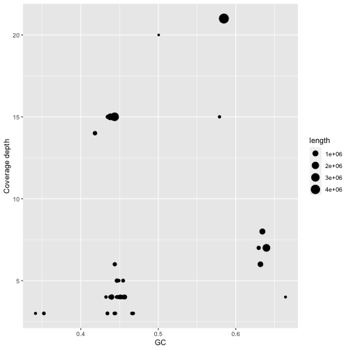
Figure 3: Coverage and GC content of assembled contigs in the mock community assembly. Contig lengths are shown through point size.

Adding labels allows us to look at the contigs with highest coverage and compare these with the contigs in bandage. Notice how the contigs for Vibrio alfacsensis cluster together.

Question 3.4

In the plot of GC versus coverage there is a cluster of contigs with high GC content (>60%) and coverage depth around 7.5x. Which species are these likely to belong to?

library(ggrepel)
gc_info %>% 
  filter(GC<0.8) %>% 
  filter(cov.<25) %>% 
  ggplot(aes(x=GC,y=cov.)) + geom_point(aes(size=length)) + geom_label_repel(aes(label=`#seq_name`))

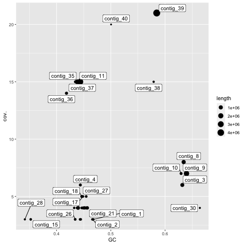Figure 4: Coverage and GC content of assembled contigs in the mock community assembly. Contig lengths are shown through point size. Only contigs with more than 25x coverage and less than 80% GC coverage are shown.

Assembly size vs reference size

Since our mock metagenome has a precisely known composition we can assess its completeness in a crude way simply by comparing the length of our assembly with that of the reference.

We will do this from within our top-level project directory. Wherever you are you can change to this directory with the following command (assuming your project was called workshop3_metasm and you put it in your home directory)

cd ~/workshop3_metasm

Firstly lets calculate the total length of our reference sequences. This command builds on one we ran earlier to list the size and GC content of reference chromosomes, but this time we have added another very simple awk program to take the sum of the second column.

cat /pvol/data/mg/refs/*.fna | bioawk -c fastx -f gc.awk | awk '{sum+=$2}END{print sum}'

Running this command should tell us that the total length of the reference is around 24Mb.

Question 3.5

Calculate the total length of your assembly using R by taking the sum of the contig lengths column. What proportion of the reference sequence does this represent?

In a real metagenomic assembly there is nothing to compare the total assembly length with so we don’t usually assess completeness this way. Later we will explore how to assess completeness for individual taxa within our assembly which is the common approach in real situations. For now, let’s continue to use the assembly length as a metric because this will allow us to explore the effect of sequencing volume on assembly completeness.

The data we have been working with so far represents 50 gigabases (Gb) of raw reads. What if we had less than this? What if we had more? How would this affect the contiguity of our assembly?

To explore these questions I have run flye on datasets with 5, 10, 20, 50, 100 and 200 gigabases of data. The results are shown in the plot below.

Activity: Think about what this plot tells us about the value of sequencing depth to metagenomic assemblies.

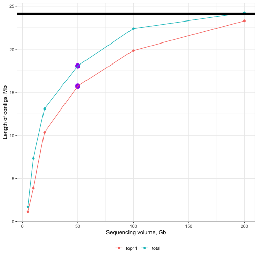
Figure 5: Effect of sequencing volume on assembly completeness. Solid black line along the top represents the size of the reference. Purple points represent the 50Gb assembly from this tutorial. Line colours differentiate between total (sum of all contigs) and top11 (sum of only the longest 11 contigs). Note that there are 11 chromosomes in the reference.

Step 4: Binning

One of the most challenging tasks in metagenomic assembly is separating sequences from the many different organisms that were present in the sample. There are many approaches to this and many different tools. Broadly speaking tools fall into two categories;

1. Read binning tools which group the raw (unassembled) reads
2. Contig binning tools which group assembled contigs

In both cases the resulting outputs are “bins” each of which will contain multiple distinct sequences (reads or contigs) that come the same organism. It is important to acknowledge that binning is a very difficult problem and the results from binning tools often contain errors such as;

1. Placing two sequences together when they come from different taxa (leads to “contamination”)
2. Failing to group sequences that come from the same taxon (lead to fragmentation)

We will perform contig binning here since we have long-reads and can rely on metaFlye to do a good job of assembling high quality contigs from a mixed collection of reads.

Firstly we will use the program metabat2. This program tries to group contigs based on nucleotide composition and read coverage. This is very similar to what we did (crudely) with our plotting approach in step 3 but uses more sophisticated clustering and looks at tetranucleotide frequency instead of just GC content.

For simplicity and speed we will use coverage information already calculated by flye and provide this to metabat.

First create a directory for our binning work and change to it. Make sure you create your metabat directory within the top-level of your project. Before running the commands below use pwd to find out where you are and navigate to the workshop3_metasm directory using cd.

mkdir metabat
cd metabat

Prepare an input file summarising read depth information for all contigs

cat ../flye/mock/assembly_info.txt  | grep -v '#' | awk '{OFS="\t";print $1,$3}' > depths.txt

Next we need to create a new version of the assembly file in which the contigs have the same order as those in the depths.txt file. We do this using a samtools faidx which allows us to extract entries from a fasta file in whatever order we specify.

cat depths.txt | awk '{print $1}' | xargs samtools faidx ../flye/mock/assembly.fasta > assembly_ordered.fasta

Finally, run metabat as follows

metabat2 -i assembly_ordered.fasta -a depths.txt --cvExt -o bins/metabat --seed 5

The bins directory will contain multi-fasta files with each of the bins inferred by metabat. To quickly inspect which contigs were grouped into which bin we can just use a grep command like this

grep '>' bins/*

You can see here that metabat has grouped contigs into 5 bins (exact numbers can vary from run to run which is why we used the --seed argument above). If you compare the contigs in these bins with those shown in bandage you can see that the largest and highest coverage contig has not been included. Other than this some of the other bins seem to make some sense. For example you should see bins that contain similar groupings of contigs to those that you explored by hand using bandage + GC content and coverage.

Step 5: Check bin quality with checkM

In this step we will use a program called checkM to assess the quality of our bins. Remember that each bin generated by metabat should represent a single species or strain within our community. Our goal is to create bins in which;

1. The sequences within the bin contain the complete sequence for this organism.
2. The sequences within the bin all come from the same organism and are not contaminated with sequences from other taxa.

We can assess the degree to which our binning and assembly has achieved these goals using checkM.

First create a working directory for running checkM and change into it. This should be very familiar by now. Make sure you are creating this directory within the top level of your project folder.

cd ~/workshop3_metasm
mkdir checkm
cd checkm

Firstly we prepare inputs for checkM. We copy over the bins from metabat

mkdir bins
cp ../metabat/bins/metabat.*.fa bins/

Remember that metabat failed to include our longest contig in bins. In my assembly this was contig_39 but for you it may be different. We need to extract this contig from our assembly and include it with our metabat bins.

samtools faidx ../flye/mock/assembly.fasta contig_39 > bins/contig_39.fa

Now run the checkm workflow. Since checkm can be very resource intensive you must run it within a slurm job script. Create a new file within your checkm directory and name it run_checkm.sh. Copy the following code into your run_checkm.sh file

#!/bin/bash
#SBATCH --time=60
#SBATCH --ntasks=4 --mem=40gb

echo "Starting checkm in $(pwd) at $(date)"

shopt -s expand_aliases
alias checkm='apptainer run -B /pvol/:/pvol /pvol/data/sif/checkm.sif checkm'

checkm lineage_wf bins out -t 4 -x fa -f checkm_results.txt

echo "Finished checkm in $(pwd) at $(date)"

Submit your job with

sbatch run_checkm.sh

And monitor progress with

tail -f slurm-XXX.out

Once checkm has finished take a look at the results file, checkm_results.txt. It provides a summary of results for each of the bins. This includes

• Marker Lineage: An approximate taxonomic classification. This is used by checkM to determine which marker genes to use for completeness and contamination checks
• # genomes: number of reference genomes used to infer marker set
• # markers: number of inferred marker genes
• # marker sets: number of inferred co-located marker sets
• 0-5+: number of times each marker gene is identified
• Completeness: estimated completeness. This is calculated by taking the number of marker genes appearing exactly 1 time and dividing by the total
• Contamination: estimated contamination. This is the number of marker genes appearing >1 times divided by the total
• Strain heterogeneity: estimated strain heterogeneity. This is calculated by examining the marker genes appearing >1 times and determining the proportion of these that are from the same or very similar organisms (strains).

Question 3.6

Which bin has the highest level of contamination? Why do you think this might be?

Application to real data: Assembling the metagenome of black band disease.

JCU PhD student Julia Hung is studying metabolic processes within the black band disease (BBD) community. In 2023 she collected fresh samples of BBD from infected individuals of the coral, Acropora hyacynthus at Orpheus Island. She successfully extracted high molecular weight DNA from these samples and sequenced them using an oxford nanopore MinION sequencer.

You have been provided with a subset of Julia’s data which should be sufficient to generate a useful metagenome assembly. We will not be working with the full dataset because the computing resources required to do so are too large for a class setting.

First switch back to the raw_data directory that you created earlier

cd ~/workshop3_metasm/raw_data

Then make a symbolic link to the bbd read data

ln -s /pvol/data/metagenome_assembly/bbd_0.1.fastq.gz .

Now switch back to the flye directory

cd ../flye

Now we will make a new copy of our run_flye.sh script with some modifications to use the black band disease data. First make a copy of the original script

cp run_flye.sh run_flye_bbd.sh

Now open the run_flye_bbd.sh script by clicking it in RStudio. This shuold bring up a text editor so you can edit the script. Edit it so it looks like this

#!/bin/bash
#SBATCH --time=360
#SBATCH --ntasks=12 --mem=10gb

echo "Starting flye bbd in $(pwd) at $(date)"

flye --nano-hq ../raw_data/bbd_0.1.fastq.gz --threads 12 --out-dir bbd --meta

echo "Finished flye bbd in $(pwd) at $(date)"

And now submit your job using

sbatch run_flye_bbd.sh

Since lots of people will be trying to run jobs on the server it is likely that yours will wait in the queue until it starts. You can check the queue with the squeue command

squeue

Take a look for your username. When your job is running the ST column will show an R (running). You will also see a new slurm-XXX.out file appear in your flye directory.

This time flye will take quite a while to run. Depending on how many people are running it at the same time it could take many hours. The recommended workflow is to start your run, monitor it for a while to make sure it is working and then allow it to run overnight.

Prior to the next workshop session you should do the following;

1. Let your flye assembly run finish
2. Run metabat on your flye assembly.

   cd ~/workshop3_metasm/metabat
   cat ../flye/bbd/assembly_info.txt  | grep -v '#' | awk '{OFS="\t";print $1,$3}' > depths_bbd.txt
   cat depths_bbd.txt | awk '{print $1}' | xargs samtools faidx ../flye/bbd/assembly.fasta > assembly_bbd_ordered.fasta
   metabat2 -i assembly_bbd_ordered.fasta -a depths_bbd.txt --cvExt -o bins_bbd/metabat --seed 5
   

3. Run checkm on the bins created by metabat. YOu will need to find the number of your largest contig in the bbd assembly and substitute for XX in the code below.

   cd ~/workshop3_metasm/checkm
   mkdir bins_bbd
   cp ../metabat/bins_bbd/*.fa bins_bbd/
   samtools faidx ../flye/bbd/assembly.fasta contig_XX > bins_bbd/contig_XX.fa
   

   Then create a slurm script for your checkm run. Your script should look like this and you should save it within your checkm directory as run_checkm_bbd.sh ```bash #!/bin/bash #SBATCH –time=60 #SBATCH –ntasks=6 –mem=10gb

echo “Starting checkm in $(pwd) at $(date)”

shopt -s expand_aliases alias checkm=’apptainer run -B /pvol/:/pvol /pvol/data/sif/checkm.sif checkm’

checkm lineage_wf bins_bbd out -t 4 -x fa -f checkm_results_bbd.txt

echo “Finished checkm in $(pwd) at $(date)”

Submit your checkm job like this
  ```bash
  sbatch run_checkm_bbd.sh